Tutorials

This section provides step-by-step tutorials for using the evolutionary optimization framework, focusing on the core functionality of the evopt package.

Basic Optimization

Single-Objective Optimization

Learn how to set up and run a basic optimization problem:

import evopt

# Define parameter space with bounds
params = {
    'x': (-5, 5),
    'y': (-5, 5),
}

# Define evaluator function (Rosenbrock function)
def evaluator(param_dict):
    x = param_dict['x']
    y = param_dict['y']
    return (1 - x)**2 + 100 * (y - x**2)**2

# Run optimization
results = evopt.optimize(
    params=params,
    evaluator=evaluator,
    batch_size=16,
    max_workers=4,
    verbose=True
)

# Print results
print(f"Best parameters: {results.best_parameters}")
print(f"Final error: {results.final_error}")

# Analyze convergence history
print(f"Epochs completed: {results.epochs_completed}")
print(f"Termination reason: {results.terminated_reason}")

Advanced Optimization

Multi-Objective Optimization with Constraints

This example demonstrates how to optimize with multiple objectives and constraints:

import evopt

# Define engineering simulation that returns multiple metrics
def structural_simulation(params):
    height = params['height']
    width = params['width']
    length = params['length']

    # Calculate metrics (in a real case, this would run your simulation)
    weight = height * width * length * 7.8  # Density of steel
    stress = 1000 / (height * width)
    deflection = 500 / (height**2 * width)

    return {
        'weight': weight,
        'stress': stress,
        'deflection': deflection
    }

# Define parameter space
params = {
    'height': (1, 10),
    'width': (1, 20),
    'length': (10, 100),
}

# Define target values with constraints
# Targets can be specified by any combination of the following formats:
    # dict[key: dict[value, hard], ...]
    # dict[key: (min, max), ...]
    # dict[key: value, ...]
    # dict[key: dict[(min, max), hard], ...]
targets = {
    'weight': {'value': 500, 'hard': False},  # Soft constraint
    'stress': (0, 50),                        # Hard constraint range
    'deflection': {'value': 1.0, 'hard': True}  # Hard constraint
}

# Run optimization
results = evopt.optimize(
    params=params,
    evaluator=structural_simulation,
    target_dict=targets,
    batch_size=32,
    max_workers=8,
    num_epochs=50
)

print(f"Best parameters: {results.best_parameters}")

Checkpointing and Resuming Optimization

Learn how to resume interrupted optimization runs:

import evopt
import os

# Define unique directory ID for this optimization
base_dir = "./optimization_studies" # Your directory for all studies
dir_id = 5  # This will create "./optimization_studies/evolve_5"

# First run (might be interrupted)
results = evopt.optimize(
    params=params,
    evaluator=evaluator,
    base_dir=base_dir,
    dir_id=dir_id,
    num_epochs=100
)

# Resume optimization from the last epoch
results = evopt.optimize(
    params=params,
    evaluator=evaluator,
    base_dir=base_dir,
    dir_id=dir_id,
)

# Resume from a specific epoch
results = evopt.optimize(
    params=params,
    evaluator=evaluator,
    base_dir=base_dir,
    dir_id=dir_id,
    start_epoch=57
)

Visualization

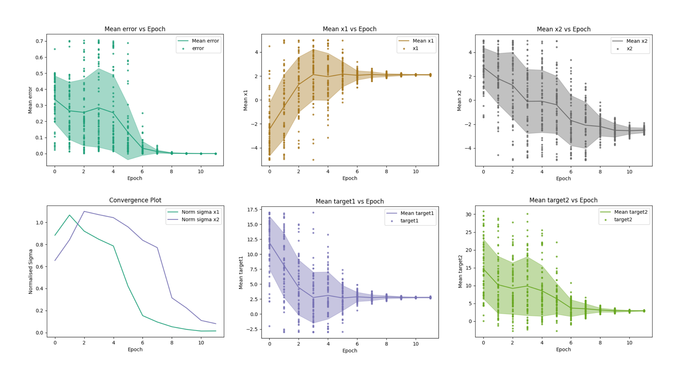
Basic Convergence Plots

Generate plots showing how parameters converged during optimization:

import evopt

# Path to optimization results
evolve_dir = "./optimization_results/evolve_5"

# Generate convergence plots
evopt.Plotting.plot_epochs(
    evolve_dir_path=evolve_dir,
    show=True,
    save_figures=True
)

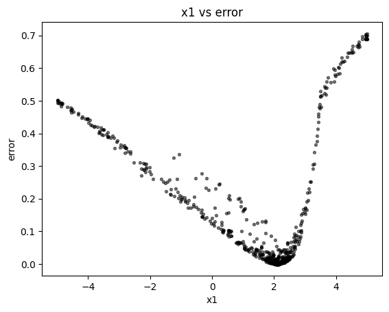
Parameter Space Visualization

Create various visualizations of the parameter space:

import evopt

evolve_dir = "./optimization_results/evolve_5"

# 2-D scatter plot (parameter vs error)
evopt.Plotting.plot_vars(
    evolve_dir_path=evolve_dir,
    x="height",
    y="error"
)

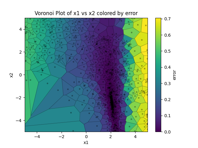
# 2-D Voronoi diagram colored by error
evopt.Plotting.plot_vars(
    evolve_dir_path=evolve_dir,
    x="height",
    y="width",
    cval="error"
)

# 3-D surface plot
evopt.Plotting.plot_vars(
    evolve_dir_path=evolve_dir,
    x="height",
    y="width",
    z="stress"
)

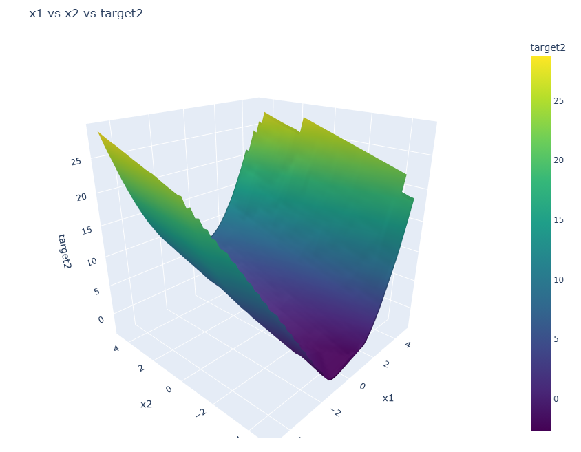
# 4-D visualization (3D surface with color)
evopt.Plotting.plot_vars(
    evolve_dir_path=evolve_dir,
    x="height",
    y="width",
    z="deflection",
    cval="epoch"
)

High-Performance Computing

Running on SLURM Clusters

The following demonstrates how to run optimizations on a SLURM-based HPC system:

Step 1: Create a simple optimization script

Create a file named optimize.py:

# filepath: optimize.py
import evopt

# Define a simple parameter space
params = {
    'x': (-5, 5),
    'y': (-5, 5),
    'z': (-5, 5)
}

# Define evaluator function
def evaluator(params):
    # This would typically call your simulation or analysis code
    x, y, z = params['x'], params['y'], params['z']
    return x**2 + y**2 + z**2  # Simple function to minimize

# Run optimization with HPC settings
results = evopt.optimize(
    params=params,
    evaluator=evaluator,
    batch_size=16,
    max_workers=8,             # Will use up to 8 parallel SLURM jobs
    hpc_cores_per_worker=2,    # Each worker gets 2 CPU cores
    hpc_memory_gb_per_worker=4,# Each worker gets 4GB RAM
    hpc_wall_time="2:00:00",   # 2-hour time limit per worker
    verbose=True
)

# Print results
print(f"Best parameters: {results.best_parameters}")
print(f"Final error: {results.final_error}")

Step 2: Create a simple SLURM submission script

Create a file named submit_job.sh:

#!/bin/bash
#SBATCH --job-name=evopt_job
#SBATCH --output=evopt_%j.out
#SBATCH --error=evopt_%j.err
#SBATCH --time=24:00:00
#SBATCH --nodes=1
#SBATCH --ntasks=1
#SBATCH --cpus-per-task=2
#SBATCH --mem=8G

# Load necessary modules
module load python

# Run the optimization script
python optimize.py

echo "Job completed"

Step 3: Submit the job

Submit your job to SLURM:

$ sbatch submit_job.sh

How it works

When you run this setup:

1. SLURM launches your main Python script

2. The evopt.optimize() function detects it’s running in a SLURM environment

3. For each batch of evaluations, evopt automatically: - Creates the necessary parameter files - Submits worker jobs to SLURM (up to max_workers) - Waits for all workers to complete - Collects and processes the results

You don’t need to manually handle the parallelization - evopt takes care of submitting the appropriate SLURM jobs based on your settings.

Note: For more complex simulations, you would typically modify the evaluator function to interact with your simulation software or external tools as needed.

Case Studies

Engineering Design Optimization

A complete example of optimizing an engineering design:

# Example of optimizing a truss structure
import evopt
import numpy as np

# Define truss simulation function
def simulate_truss(params):
    # In a real case, this would call an engineering simulation software
    # For this example, we'll use a simplified model

    # Extract design parameters
    cross_section = params['cross_section']
    height = params['height']
    span = params['span']

    # Calculate performance metrics
    material_volume = cross_section * (span + 2 * height)
    max_stress = 1000 * span / (cross_section * height)
    deflection = span**3 / (48 * 200e9 * cross_section * height**2)

    return {
        'volume': material_volume,
        'stress': max_stress,
        'deflection': deflection
    }

# Define parameter space
params = {
    'cross_section': (0.001, 0.01),  # m2
    'height': (0.5, 2.0),           # m
    'span': (5.0, 15.0)             # m
}

# Define targets
targets = {
    'volume': {'value': 0.1, 'hard': False},      # Minimize volume (soft)
    'stress': (0, 250e6),                         # Stress limit (hard)
    'deflection': {'value': 0.01, 'hard': True}   # Deflection limit (hard)
}

# Run optimization
results = evopt.optimize(
    params=params,
    evaluator=simulate_truss,
    target_dict=targets,
    batch_size=32,
    max_workers=8
)

# Visualize results
evolve_dir = f"./evolve_{results.directory_id}"
evopt.Plotting.plot_epochs(evolve_dir)
evopt.Plotting.plot_vars(evolve_dir, x="cross_section", y="height", cval="volume")

Machine Learning Hyperparameter Optimization

Optimize hyperparameters for a machine learning model:

import evopt
from sklearn.ensemble import RandomForestClassifier
from sklearn.datasets import load_iris
from sklearn.model_selection import cross_val_score

# Load data
iris = load_iris()
X, y = iris.data, iris.target

# Define evaluator function
def evaluate_model(params):
    # Create model with parameters
    model = RandomForestClassifier(
        n_estimators=int(params['n_estimators']),
        max_depth=int(params['max_depth']),
        min_samples_split=int(params['min_samples_split']),
        random_state=42
    )

    # Evaluate using cross-validation
    scores = cross_val_score(model, X, y, cv=5)
    # Return negative score because we're minimizing
    return -scores.mean()

# Define parameter space
params = {
    'n_estimators': (10, 200),
    'max_depth': (3, 20),
    'min_samples_split': (2, 20)
}

# Run optimization
results = evopt.optimize(
    params=params,
    evaluator=evaluate_model,
    batch_size=16,
    max_workers=4,
    num_epochs=20
)

print("Best hyperparameters:")
for param, value in results.best_parameters.items():
    if param in ['n_estimators', 'max_depth', 'min_samples_split']:
        print(f"{param}: {int(value)}")

print(f"Best accuracy: {-results.final_error:.4f}")

Symbolic Regression

Equation Discovery with PySR

Learn how to discover mathematical equations from data using symbolic regression:

import evopt
import matplotlib.pyplot as plt

# Initialize the Derive class with existing data
# Assumes results.csv exists in the specified directory with columns x1, x2, x3, and y
model = evopt.Derive(
    evolve_dir_path="./simulation_results/evolve_5",
    target_variable="y",
    parameters=["x1", "x2", "x3"],
    unary_operators=["sin", "cos", "exp"],  # Include trigonometric functions
    n_iterations=40,                        # Number of iterations
    population_size=32,
    max_size=20                            # Maximum equation complexity
)

# Fit the model to discover equations
model.fit()

# Print the best equation found
print(f"Discovered equation: {model.best_equation}")

# Make predictions using the discovered equation
model.predict()

# Create a parity plot to visualize the fit
model.parity_plot(
    point_colour="blue",
    alpha=0.6,
    title="Actual vs. Predicted Values",
    save_figures=True,
    show=True
)